Natural language search in Google BigQuery
How to build a semantic search and related articles tool in BigQuery using word vectors
This tutorial explains how to build a simple, but powerful, natural language search facility in BigQuery using only Standard SQL and freely available pre-trained word vectors. In the worked example, I use a dataset of 125,000 articles from various Nature journals included in Google’s Breathe project, and accessible from the bigquery-public-data project in the BigQuery console.
Why BigQuery? It’s easy to find tutorials and libraries that will let you build similar document search tools in Python, so why bother doing it in SQL? The answer is that it extends the range of analysis that you can undertake without leaving the BigQuery ecosystem: you can do relatively sophisticated NLP tasks entirely in SQL. This saves you the trouble of importing and exporting between BigQuery and a Python instance, and gets everything done in one place.
It certainly isn’t going to be the right solution in many cases, but as with BigQuery ML, it’s a useful addition to your toolkit.
Running the tutorial
All the code for the tutorial can be found in this github repo.
To get the code to run you will need to create a Google cloud project, and enable billing for BigQuery. Google currently provides 10GB of storage and 1TB per month of query processing for free. So, with a bit of care, you will be able to run the tutorial without incurring having to pay anything. Without due care, you could potentially rack up a small bill since we are dealing with quite large amounts of data. The word vectors used in the tutorial take up 5GB of storage, and each query using this dataset therefore uses 5GB of processing capacity, i.e. 200 queries before the free allowance runs out. There are some suggestions on reducing query costs at the end of the article.
Word vectors for natural language document search
A word vector is a numeric representation of a word. It maps words to locations in a multi-dimensional space. The magic of these pre-trained word vectors is that the mapping contains some knowledge of the context in which the words have been used. Words that could plausibly be substituted for one another tend to be located close together in the word vector space.
This feature allows us to build a sophisticated document search engine: one which gives the impression of knowing the meaning of the documents rather than just finding keywords.
In outline, the steps to build a SQL based natural language search tool are as follows:
Import pre-trained word vectors to BigQuery;
Convert each document we want to be able to search to a single vector and save these in a table;
Convert the search phrase to a vector;
Calculate the distance between the search vector and all the stored document vectors;
Rank the documents according to this distance — shorter distance implies a better match.
The rest of the article goes through each step, providing code examples.
1. Import word vectors to BigQuery
The first step is to import some pre-trained word vectors into BigQuery. I’ve chosen to use the cased 300 dimension Glove vectors trained on a huge dataset of text scraped from the web (https://nlp.stanford.edu/data/glove.840B.300d.zip). This contains vectors for over 2.2 million distinct “words”. [Strictly speaking we should call these “tokens” and not “words”, since the vocabulary will include things like numbers, dates, abbreviations. For the remainder, I use word and token interchangeably.]
Table schema
Each vector consists of 300 numbers (one for each of the 300 dimensions). I have chosen to store these numbers as arrays. In the Python BigQuery API, we define an ARRAY data type by setting the mode parameter of the SchemaField object to 'REPEATED':
bigquery.SchemaField("vector",
                     bigquery.enums.SqlTypeNames.FLOAT,
                     mode='REPEATED')
We could have chosen to save each element of the vector to a separate field (e.g. vec1, vec2, … vec300). However, we would then need to write out each of these fields in any query using the word vectors, which creates very wordy query text. Using arrays means the queries are much more concise and readable.
Vector import
The process I have used is to first load the vectors into a pandas dataframe, and then to use the BigQuery python API method load_table_from_dataframe to upload to a database table. (Colab crashed when I tried to save all 2.2M word vectors in one go, so I split it into batches of 250,000.)
The complete code for the import can be found in this notebook.
Once this step is complete, we have a table with 2.2M rows — one for each word — with each row containing a word and its vector stored as an array. In the BigQuery console it will look something like this:

Running a word similarity query
Now that we have the vectors in BigQuery, we can run a word similarity query. The basic idea behind similarity queries is that we compare some measure of the distance between vectors. That is, we find the words which are ‘closest’ to each other in the vector space; and infer that the closer two words are, the more similar they will be.
We could calculate Euclidean distance, but a more common approach is to use cosine similarity. This is just the cosine of the angle between two vectors. It gives you a more intuitive scale than Euclidean distance, with results between -1 and 1. A score of 1 means identical and zero implies completely different. (-1 would mean a vector pointing in the opposite direction, but note that it doesn’t imply opposite in meaning).
The maths is straightforward. A dot product is defined geometrically as:
u⋅v = ∥u∥ ∥v∥ cos θ
Where ∥u∥ and ∥v∥ and the magnitudes of vectors u and v. We can rearrange to get cos θ, and the other elements of the equation are easy to calculate in SQL from the vector components stored within arrays.
We end up with something like the following:
SELECT
 #  u⋅v / (∥u∥ * ∥v∥)
  SUM(av_component * sv_component) /
 (
    SQRT(SUM(av_component * av_component)) *
      SQRT(SUM(sv_component * sv_component))
  )
FROM
  UNNEST(all_vectors.vector)   av_component WITH OFFSET av_component_index
JOIN
  UNNEST(search_vector.vector) sv_component WITH OFFSET sv_component_index
ON av_component_index = sv_component_index
Note that you have to line up the vector components by their array offset when using UNNEST. By default, BigQuery will not preserve the order of the element in the array, and so the vector dimensions would end up being muddled.
If we normalise the vectors stored in a BigQuery table to unit length, the maths ends up a bit simpler. Both ∥u∥ and ∥v∥ would then equal 1, and so we can cancel out that part of the query. The imported Glove vectors are not normalised, so we will stick with the code above for the time being.
The following SQL gives a complete example of how to find the 10 most similar words to “apple”.
WITH
  glove AS (SELECT * FROM `{your_project_id}.word_vectors_us.glove_vectors`),

  search_vector AS (SELECT * FROM  glove
            WHERE word = 'apple'),

  cosine_sim AS (
      SELECT
          all_vectors.word,
          (SELECT #  u⋅v / (∥u∥ * ∥v∥)
              SUM(av_component * sv_component) /
             ( SQRT(SUM(av_component * av_component)) *
                  SQRT(SUM(sv_component * sv_component)) )
            FROM
              UNNEST(all_vectors.vector)   av_component WITH OFFSET av_component_index
            JOIN
              UNNEST(search_vector.vector) sv_component WITH OFFSET sv_component_index
            ON av_component_index = sv_component_index
          ) AS cosine_similarity
    FROM glove AS all_vectors
    CROSS JOIN search_vector
  )

SELECT * FROM cosine_sim
ORDER BY cosine_similarity DESC
LIMIT 10
Which gives you the following results:

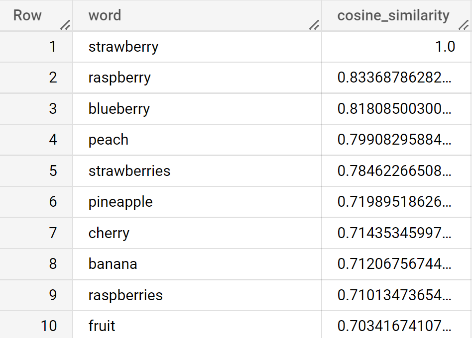
Note that word vectors capture two common uses of the word apple — both as a fruit and as a company. A query for “strawberry” produces the following:
Also, note again that the word vectors are cased, and so we get quite different results if we search for “Apple”:

2. Create document vectors
In steps 2 and 3 we need to convert a body of text into a vector. This entails the following steps:
split the text up into tokens (i.e. words);
remove stop words (very common words like ‘a’, ‘the’, ‘it’, etc);
look up the vector for each word from the pre-trained list;
produce a single vector by taking a weighted average over all the matched words vectors.
Tokenisation
The first step, tokenisation, is something that we are going to be doing repeatedly. To extract tokens from a block of text we use a regular expression, and for convenience we save the relevant SQL code as a user-defined function (UDF):
CREATE OR REPLACE FUNCTION
          `{your_project_id}.word_vectors.tokenise_text`(text STRING) AS (
(
    SELECT REGEXP_EXTRACT_ALL(
              REGEXP_REPLACE(text, r'’|\'s(\W)', r'\1'),
                             r'((?:\d+(?:,\d+)*(?:\.\d+)?)+|(?:[\w])+)')
    )
);
If you are not familiar with regular expressions, this will look a bit cryptic. The first part strips apostrophes from words. The second bit then extracts anything matching one of two patterns:
(:\d+(?:,\d+)*(?:\.\d+)?)should capture numbers, including sequences of numbers with commas and a full stop as a decimal point such as “12,345.78”. Note that this isn’t very strict and will allow comma separated lists e.g. “10,20,30,40,50”.(?:[\w])+just means extract any continuous set of word characters, i.e. anything that isn’t for example a punctuation mark or space.
The UDF above will return an array containing all the tokens in the text. To look up the matching word vectors we simply JOIN to the word vector table.
Remove stopwords
You don’t have to remove stopwords, but it does tend to produce better results. Given that we will need to do this every time we tokenise some text, it makes sense to add this to the UDF. Rather than store the stopwords in a small table, we can just add them to the UDF code itself. A long list of stopwords does mean a very wordy query, but it’s all hidden inside the function, so this doesn’t really matter.
CREATE OR REPLACE FUNCTION `{your_project_id}.word_vectors_us.tokenise_no_stop`(text STRING) AS (
(
    SELECT ARRAY_AGG(word) FROM UNNEST(REGEXP_EXTRACT_ALL(
                                REGEXP_REPLACE(text, r'’|\'s(\W)', r'\1'),
                                r'((?:\d+(?:,\d+)*(?:\.\d+)?)+|(?:[\w])+)')) AS word
    WHERE LOWER(word) not in UNNEST(['a', 'about', 'above', 'after', 'again', 'against', 'ain', 'all', 'am', 'an', 'and', 'any', 'are', 'aren', 'arent', 'as', 'at', 'be', 'because', 'been', 'before', 'being', 'below', 'between', 'both', 'but', 'by', 'can', 'couldn', 'couldnt', 'd', 'did', 'didn', 'didnt', 'do', 'does', 'doesn', 'doesnt', 'doing', 'don', 'dont', 'down', 'during', 'each', 'few', 'for', 'from', 'further', 'had', 'hadn', 'hadnt', 'has', 'hasn', 'hasnt', 'have', 'haven', 'havent', 'having', 'he', 'her', 'here', 'hers', 'herself', 'him', 'himself', 'his', 'how', 'i', 'if', 'in', 'into', 'is', 'isn', 'isnt', 'it', 'its', 'itself', 'just', 'll', 'm', 'ma', 'me', 'mightn', 'mightnt', 'more', 'most', 'mustn', 'mustnt', 'my', 'myself', 'needn', 'neednt', 'no', 'nor', 'not', 'now', 'o', 'of', 'off', 'on', 'once', 'only', 'or', 'other', 'our', 'ours', 'ourselves', 'out', 'over', 'own', 're', 's', 'same', 'shan', 'shant', 'she', 'shes', 'should', 'shouldn', 'shouldnt', 'shouldve', 'so', 'some', 'such', 't', 'than', 'that', 'thatll', 'the', 'their', 'theirs', 'them', 'themselves', 'then', 'there', 'these', 'they', 'this', 'those', 'through', 'to', 'too', 'under', 'until', 'up', 've', 'very', 'was', 'wasn', 'wasnt', 'we', 'were', 'weren', 'werent', 'what', 'when', 'where', 'which', 'while', 'who', 'whom', 'why', 'will', 'with', 'won', 'wont', 'wouldn', 'wouldnt', 'y', 'you', 'youd', 'youll', 'your', 'youre', 'yours', 'yourself', 'yourselves', 'youve'])
    )
);
Count word frequencies
The final step is to take an average over all the matched word vectors in the document. This will squash the amount of information we retain about the document down to the equivalent of a single word. Not all words convey the same amount of information, and we want to try to capture the essence of the text. This is why we have already removed stopwords, but we would also like to give more weight to more important words.
We can use a trick borrowed from an (even) older NLP technique — inverse frequency weighting. When taking the average, we weight each vector according to the inverse of that word’s frequency in all the documents in our corpus. More common words receive less weight, and conversely, those we don’t see very often will be deemed more important.
We can use SQL to find these word frequencies: tokenise all the documents using our UDF; UNNEST all the resulting arrays into one long list of tokens; and then count them. Since we are going to be using these word frequencies every time we run a similarity query, it makes sense to save them to a table. The following SQL will create this table:
CREATE OR REPLACE TABLE
    `{your_project_id}.word_vectors_us.word_frequencies` AS

WITH tokens AS (
  SELECT `{your_project_id}.word_vectors_us.tokenise_text`(body) AS tk
  FROM `bigquery-public-data.breathe.nature`
)
SELECT w AS word, COUNT(*) AS frequency
FROM tokens, UNNEST(tk) AS w
GROUP BY 1
Document vector calculation
One more decision to make is how exactly to weight the vectors. We could weight by inverse frequency, but in a large corpus this could significantly downweight some important words.
Remember that weighting is relative: if one word appeared 50,000 times, and another only 10 times, the more common word would be deemed 5,000 times less important. After some very unscientific messing around, I settled for a weighting of 1 / frequency^.4. This sits somewhere between inverse frequency (too much weight for rare words) and log(frequency) (too much weight for common words).
The overall conclusion is that you should downweight high frequency words and upweight low frequency ones, but the exact weighting is something you can experiment with.
Normalise the vectors to unit length
Once you have settled on a weighting, the final step is to normalise the vectors. From an arithmetic point of view, we don’t need to worry about choosing weights which add up to 1: we simply choose a set of weights with appropriate relative values; and then normalise the vector to unit length. As noted above, saving normalised vectors also then simplifies the subsequent calculations of cosine similarity.
The following code combines all these steps to calculate document vectors for all the body text of the Nature articles in the breathe dataset, and save them to our dataset:
CREATE OR REPLACE TABLE `{your_project_id}.word_vectors_us.nature_vectors`
AS

WITH all_articles AS (SELECT  id,
                              date,
                              title,
                              `{your_project_id}.word_vectors_us.tokenise_no_stop`(body) article

FROM `bigquery-public-data.breathe.nature`),

# Unnest so we have one word per row
my_word_lists AS (
            SELECT  id,
                    word
            FROM all_articles, UNNEST(article) AS word
   ),

# Fetch the vectors for each word and weight by word frequency
lookup_vectors AS (
  SELECT
        id,
        word,
        wv_component / POW(frequency, 0.4) AS tf_normalised_wv_component,
        wv_component_index
  FROM my_word_lists
  JOIN `{your_project_id}.word_vectors_us.glove_vectors`
    USING (word)
  JOIN `{your_project_id}.word_vectors_us.word_frequencies`
    USING (word)
  , UNNEST(vector) wv_component WITH OFFSET wv_component_index),

# Aggregate to create a document vector
aggregate_vectors_over_article AS (
  SELECT   id,
           wv_component_index,
           SUM(tf_normalised_wv_component) aggregated_wv_component
  FROM lookup_vectors
  GROUP BY id, wv_component_index),

# Normalise vectors to unit length, so need to work out the length (magnitude)
vector_lengths AS (
  SELECT id,
         SQRT(SUM(aggregated_wv_component * aggregated_wv_component)) AS magnitude
  FROM aggregate_vectors_over_article
  GROUP BY id),

# Divide by the magnitude to normalise and put it back in to an array
normalised_aggregate_vectors AS (
    SELECT id,
           ARRAY_AGG(aggregated_wv_component / magnitude ORDER BY wv_component_index) AS article_vector
    FROM aggregate_vectors_over_article
    JOIN vector_lengths
      USING (id)
    GROUP BY id)

SELECT  id,
        date,
        title,
        article_vector
FROM normalised_aggregate_vectors
JOIN all_articles
USING (id)
The query is doing a lot of work, and so will take quite a long time to run (around 15 minutes). For each of the 125k Nature articles, it is tokenising the text, looking up word vectors for each token, and then calculating a weighted average document vector. (Just to note, the resulting table contains 113k document vectors. Some of the entries in the source table do not contain any body text.)
3. Create a search vector
The next step is to generate a search vector which we will then compare to the document vectors created in the previous step. We use exactly the same steps as performed before to create document vectors: tokenise the search phrase; remove stop words; look up word vectors and then calculate a weighted average. The only change required to the code is to use the search phrase as the text input rather than the text of an article.
4. Perform the search
Here we run the same kind of query we ran earlier to find similar words, but this time we compare the pre-calculated document vectors with the search vector. Also, since we have normalised both the document vectors and the search vector, we only need calculate a dot product to find the cosine similarity:
SELECT SUM(doc_vector_component * search_vector_component)
FROM
  UNNEST(dv.vector) doc_vector_component WITH OFFSET dv_component_index
JOIN
  UNNEST(s.vector) search_vector_component WITH OFFSET sv_component_index
ON dv_component_index = sv_component_index
5. Rank results according to cosine similarity
The final step is simply to rank the results according to descending cosine similarity, and pull in any additional fields of data to make the search results useful.
The complete similarity search query is quite long, and so for convenience we can save it as a stored procedure. Note that the final LIMIT statement controls how many search results are presented.
CREATE OR REPLACE PROCEDURE `{your_project_id}.word_vectors_us.similarity_search`(search_phrase STRING)
BEGIN

WITH
  all_tokens AS (SELECT  `{your_project_id}.word_vectors_us.tokenise_no_stop`(search_phrase) tokens),

  # Unnest so we have one word per row
  tokens_no_stops AS (
            SELECT  word
            FROM all_tokens, UNNEST(tokens) AS word
   ),

  # Fetch vectors for each word, and weight by the word frequency in the corpus
  lookup_vectors AS (SELECT
                            word,
                            vector_component / POW(frequency, 0.4) AS weighted_vector_component,
                            vector_component_index
  FROM tokens_no_stops
  JOIN `{your_project_id}.word_vectors_us.glove_vectors`
  USING (word)
  JOIN `{your_project_id}.word_vectors_us.word_frequencies`
  USING (word)
  ,
  UNNEST(vector) vector_component WITH OFFSET vector_component_index),

  # Aggregate the weighted components to generate a single vectors. Just take the SUM
  aggregate_vector AS (SELECT vector_component_index, SUM(weighted_vector_component) AS agg_vector_component
                    FROM lookup_vectors
                    GROUP BY vector_component_index),

  # We want to normalise the vectors to unit length, so need to work out the length (magnitude) of the
  vector_length AS (SELECT SQRT(SUM(agg_vector_component * agg_vector_component)) AS magnitude
  FROM aggregate_vector),

  # Divide by the magnitude to normalise and put it back in to an array
  norm_vector AS (
    SELECT ARRAY_AGG(agg_vector_component / (SELECT magnitude FROM vector_length) ORDER BY vector_component_index) AS vector
    FROM aggregate_vector)

SELECT  id,
        date,
        title,
        (SELECT SUM(doc_vector_component * search_vector_component)
         FROM
            UNNEST(dv.article_vector) doc_vector_component WITH OFFSET dv_component_index
         JOIN
            UNNEST(s.vector) search_vector_component WITH OFFSET sv_component_index
         ON dv_component_index = sv_component_index) AS cosine_similarity
FROM `{your_project_id}.word_vectors_us.nature_vectors` dv
CROSS JOIN norm_vector s
ORDER BY cosine_similarity DESC
LIMIT 10;
END;
To run a similarity query we just CALL this procedure.
We can now test it by searching using the title of one of the articles in the dataset as our query text:
CALL `{your_project_id}.word_vectors_us.similarity_search`(
  "Epigenetics and cerebral organoids: promising directions in autism spectrum disorders"
);
This produces the following results:

The top result is the article we searched for, and the remaining results seem to be relevant. It’s rather difficult to tell given the technical nature of the articles. Note that the cosine similarity is considerably less than 1 for the source article. This is because we are comparing the similarity of its title to the body text.
If we used the complete body text for the search we get different results. This is the equivalent to finding the most closely related articles. Let’s look at this problem in the final section.
Finding related articles
Since we have already calculated all the document vectors, we don’t need to tokenise and look up and word vectors. We use pretty much the same code, but simply look up the search vector from the precalculated table of document vectors.
WITH
  search_vector AS (
SELECT article_vector AS vector
  FROM `{your_project_id}.word_vectors_us.nature_vectors`
  where id = "5de2010b-bee3-4669-aa24-8287a8ab6fd9" )

SELECT id,
        date,
        title,

(SELECT SUM(doc_vector_component * search_vector_component)
FROM
  UNNEST(dv.article_vector) doc_vector_component WITH OFFSET dv_component_index
JOIN
  UNNEST(s.vector) search_vector_component WITH OFFSET sv_component_index
ON dv_component_index = sv_component_index) AS cosine_similarity
FROM `{your_project_id}.word_vectors_us.nature_vectors` dv
CROSS JOIN search_vector s
ORDER BY cosine_similarity DESC
LIMIT 10;
This time the cosine similarity of the top result is 1: we are comparing the document vector to itself.

Reducing query costs
Whenever we have to tokenise and look up vectors for a new passage of text, we have to scan the entire 5GB table of Glove vectors. If you are on flat rate billing, then this isn’t really an issue; but if you pay as you go, then the costs could start to mount quite quickly. So, is there anything we can do to reduce this 5GB per query cost?
Yes, there are several approaches. The simplest option is to use a different set of pre-trained word vectors. The set we are using has a vocabulary of 2.2M cased tokens (so, “Apple” is different to “apple”), and the vectors have 300 dimensions. The Glove project also includes a set of uncased vectors with just 400k uncased tokens, which is available with as low as 50 dimensions. The downside is that these were trained on a smaller text corpus, and so perhaps not as good when applied to niche sets of documents like the ones we are using in this tutorial.
A different approach would be to use the same set of Glove vectors, but to reduce the vocabulary. There are 325k tokens which include a non-word character, e.g. hyphenated words and abbreviations with full stops. Given that our tokeniser only admits sequences of alphanumeric word characters, these tokens will never be used by our process, so we can very safely drop them. (However, this does also suggest we perhaps ought to revise the regex in our tokeniser to allow for hyphenated words.)
In addition, there are another 194k tokens which contain numbers. Most of these are numbers, but you also find things like ‘34th’, ‘100mm’, and ‘10AM’; as well as more esoteric stuff like ‘win7’, or ‘U2’.
It seems reasonable to assume that these tokens will make little difference to the precision of a document vector which is a compressed representation of 1,000+ words. There will of course be exceptions, but most of the time you will get the gist of the document from the remaining words.
Finally, if our corpus is reasonably large (like the one we are using in this example), then we could identify the vocabulary which appears in our corpus, and then just use this subset of word vectors. In this case we would end up with about 400k tokens. This would reduce the cost of a query down to about 1GB. The trade off is that you may have vocabulary in your search phrase that doesn’t appear in the corpus, but is in the original set of Glove vectors.
Final thoughts
This article has explained how you can create a natural language search tool using only SQL in BigQuery. It has also shown how to use the same document vectors to create a ‘related articles’ feature. With use of scheduled queries, you can easily build a process to keep the document vector indexes up-to-date.
An interesting extension of these techniques is to build a topic model using BigQuery ML. The code is a bit convoluted, but you can use the vector components as inputs to a logistic regression model. This can generate a quite powerful topic model which will transfer well to new texts.
Finally, it’s worth noting that the Glove vectors were trained back in 2014. Vocabulary from more recent history (e.g. “Covid19”) will be missing entirely, and the context of many other words will have changed. If you have a large enough corpus, it is probably worth training your own word vectors. Perhaps the topic for another blog post.